
Five modern Excel formulas every analyst should know
XLOOKUP, SUMIFS, LET, FILTER and TEXTSPLIT replace whole workflows. Worked examples for each, the mistakes to avoid, and which Excel versions have them.
Excel has added functions over the last few years that make older patterns unnecessary: nested
VLOOKUPs, helper columns, and the Text to Columns wizard. These five cover a large share of everyday analysis.
Each one below comes with a small worked example you can paste into a blank sheet.
1. XLOOKUP: one lookup instead of three
XLOOKUP finds a value in one column and returns the matching value from another. It replaces VLOOKUP,
HLOOKUP and most INDEX/MATCH combinations.
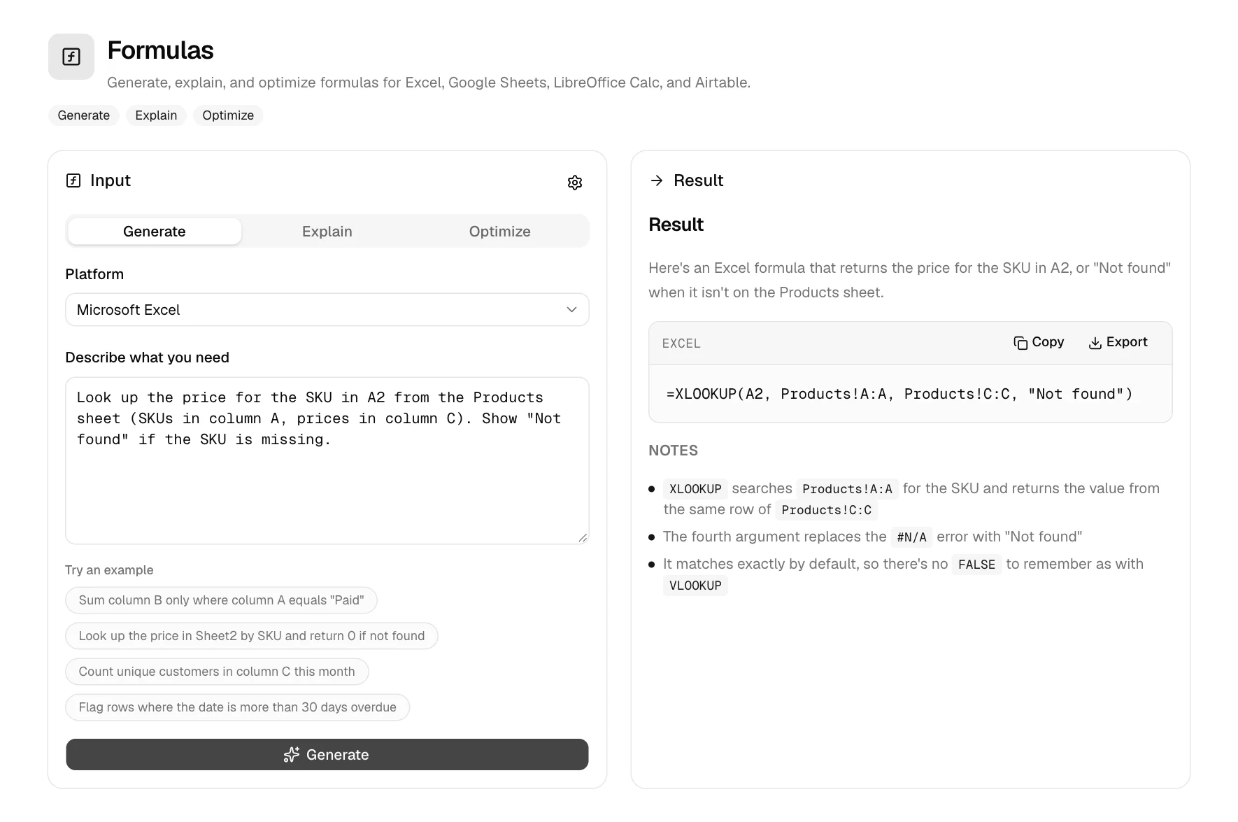
Say the Products sheet lists SKUs in column A and prices in column C, and your orders have a SKU in A2:
=XLOOKUP(A2, Products!A:A, Products!C:C, "Not found")Why it's better than VLOOKUP:
- It matches exactly by default, so there's no
FALSEto forget. - The return column can sit to the left of the lookup column.
- Inserting a column in the middle doesn't break it, because there's no column number to count.
- The fourth argument replaces
#N/Awith your own text.
2. SUMIFS: totals with conditions
SUMIFS adds up the rows that meet every condition you give it. Note the order: the column to add comes
first, then pairs of range, condition.
| A | B | C | |
|---|---|---|---|
| 1 | Region | Units | Revenue |
| 2 | West | 120 | 3,600 |
| 3 | East | 150 | 4,500 |
| 4 | West | 80 | 2,400 |
| 5 | West | 210 | 6,300 |
=SUMIFS(C2:C5, A2:A5, "West", B2:B5, ">100")The result is 9,900: rows 2 and 5 match, and row 4 is West but only 80 units. COUNTIFS and
AVERAGEIFS take the same arguments when you need a count or an average instead.
3. LET: name the parts of a long formula
LET gives names to intermediate results, so a long formula reads like a short calculation and each part
is computed once. With a price in B2 and a discount in C2:
=LET(net, B2 - C2, tax, net * 15%, net + tax)With a price of 200 and a discount of 20, net is 180, tax is 27, and the result is 207. Without LET
you'd write B2 - C2 twice, and change it in two places later.
4. FILTER: every matching row, not just the first
A lookup returns one match. FILTER returns all of them, as a live table that spills into the cells below:
=FILTER(A2:D100, C2:C100 = "Open", "No open tickets")Two things to know:
- Leave room for the results. If a value is in the way, you get
#SPILL!. - Without the third argument, a filter with no matches returns
#CALC!.
Combine conditions by multiplying them (both must be true) or adding them (either can be true):
(C2:C100 = "Open") * (D2:D100 > 5).
5. TEXTSPLIT: Text to Columns as a formula
TEXTSPLIT breaks text apart at a delimiter. With Smith, Jane, London in A2:
=TEXTSPLIT(A2, ", ")The result spills across three cells: Smith, Jane, London. Unlike the Text to Columns wizard, it
updates when A2 changes. A third argument splits into rows as well, for text like a,b;c,d.
Which versions have them
| Function | Excel 365 | Excel 2024 | Excel 2021 | Google Sheets |
|---|---|---|---|---|
| XLOOKUP | Yes | Yes | Yes | Yes |
| SUMIFS | Yes | Yes | Yes | Yes |
| LET | Yes | Yes | Yes | Yes |
| FILTER | Yes | Yes | Yes | Yes, as FILTER(range, condition) |
| TEXTSPLIT | Yes | Yes | No | Use SPLIT |
On Excel 2019 or earlier, only SUMIFS is available. Tell GPTExcel which version you use and it writes the
formula with functions you have.
Picking the right one
Let GPTExcel write them
You don't have to memorize any of this. In the Formulas tool, describe the result you want and get the formula with a note on how it works:
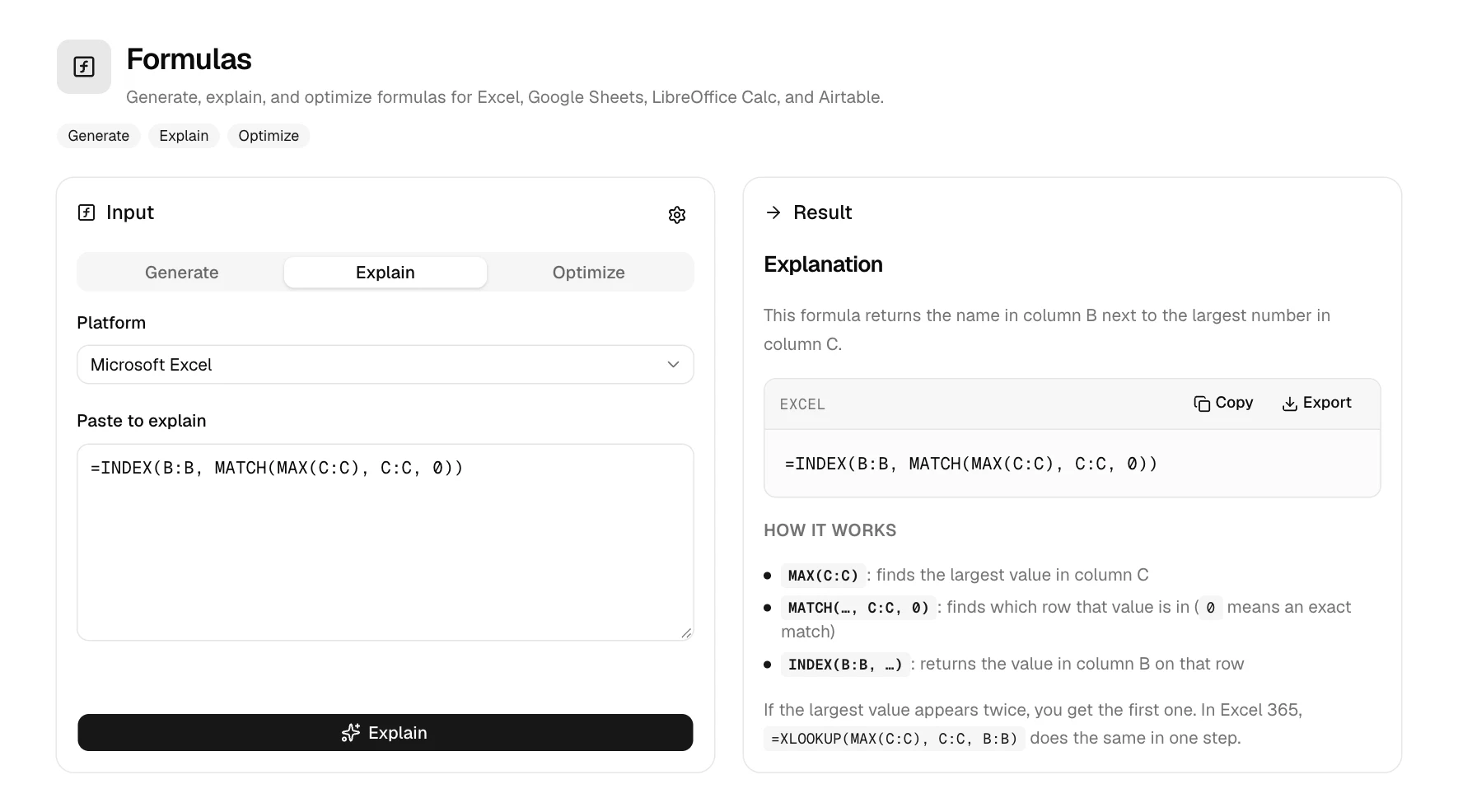
It works the other way too. Paste a formula you inherited and switch to Explain:
Set your platform (Excel, Google Sheets, LibreOffice Calc or Airtable), version and argument separator once with the settings button, and every formula follows them.